Mastering machine learning algorithms is not a myth. For most machine learning beginners, the regression algorithm is the first type of algorithm that many people come into contact with. It is easy to understand and easy to use. It is a great artifact in learning, but is it really a panacea? Through this article, IWC hopes that everyone understands that sometimes some of the most powerful tools in life are not our only choice.
If machine learning is viewed as an armory full of swords, axes, bows, and other weapons, there are tens of thousands of tools. Our choice is indeed great, but we should learn to be at the right time and place. Use the right weapon. If the regression algorithm is regarded as one of the swords, it can easily penetrate the armor of the enemy (data), but it cannot be used by Kenting to solve the cow. For highly complex data processing tasks of this type, a sharp “knifeâ€â€”support vector machine (SVM)—is often more effective—it can work on smaller data sets and build more powerful models.
1. What is a support vector machine?
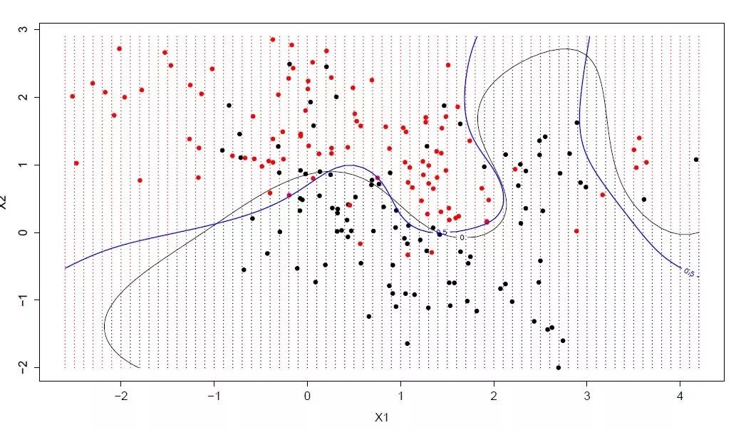
In the field of machine learning, support vector machines (SVMs) are an algorithm that can be used for classification and regression tasks to supervise learning. In practice, its main application scenario is classification. To explain this algorithm, first of all we can imagine a lot of The data, each of which is a point in a high-dimensional space, has the characteristics of the data and the number of dimensions of the space. Correspondingly, the position of the data is the coordinate value of each corresponding feature. It is possible to classify these data points perfectly. We will use the SVM algorithm to find this hyperplane.
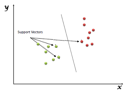
In this algorithm, the so-called "support vector" refers to the training sample points at the edge of the interval, and the "machine" is the best decision boundary for the classification (line/plane/hyperplane).
2. How SVM Works
Below we use images to demonstrate several ways to find the correct hyperplane.
Scenario 1
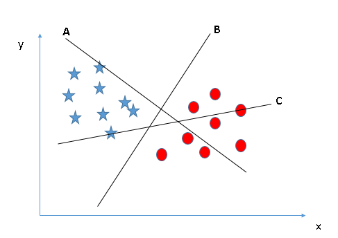
There are three hyperplanes in the figure below: A, B, and C. Which of these is the correct border? Just keep in mind that the SVM selects decision boundaries that can categorize both types of data. Obviously, compared to A and C, B better classifies circles and stars so it is the correct hyperplane.
Scenario 2
In the figure below, there are also three hyperplanes A, B, and C. This is different from scenario 1. This time, the three hyperplanes have completed the classification well. Which one is the correct hyperplane? In this regard, we revisited the previous statement: SVM selects decision boundaries that can better classify two kinds of data.
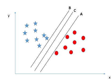
Here, we can draw the distance from the data to the decision boundary to assist in the judgment. As shown in the figure below, both stars and circles have the longest distance to C, so here C is the best decision boundary we are looking for.
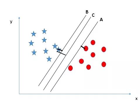
The reason why the hyperplane with farther margins is chosen is because it is more robust and its fault-tolerance rate is higher. If you choose A or C, if we continue to enter samples later, they are more likely to be misclassified.
Scenario 3
Here we look at the map first and try to make a choice based on the conclusion of the previous scenario.
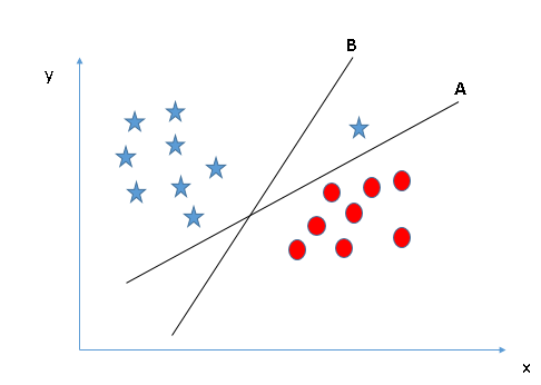
Perhaps some readers eventually chose B, because the two types of data and its margins are more distant than A. However, there is a problem that B is not classified correctly and A is correctly classified. So in front of the SVM algorithm, the correct classification and the maximum margins are heavy and light? Obviously, the SVM first considers the correct classification and the second is the optimization of the distance from the data to the decision boundary. The correct hyperplane for scenario 3 is A.
Scenario 4
In the previous examples, although we described the decision boundaries as hyperplanes, they are all straight lines in the image. This is actually not realistic. As in the figure below, we cannot use straight lines for classification.
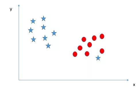
A blue star appears between the red dots and it is not on the same side as other similar data. So do we want to draw a curve to classify? Or, do you want to separate it from the atmosphere? the answer is negative.
Contrasting Scenario 3, we can infer that the star here is an anomaly, so here the SVM algorithm is not plagued by the premise of classification and we can find a most suitable hyperplane directly between the circle and the star for classification. In other words, SVM is valid for outliers.
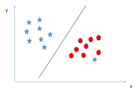
Scenario 5
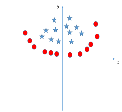
Let us continue to focus on the topic of straight lines. In the following figure, there is already no linear boundary between the two types of data. What is the classification of the SVM algorithm? Please imagine the heroes of the TV drama table shaking the glass. In the figure, there are currently only X and Y features. To classify, we can add a new feature Z = X2 + Y2 and plot the data points on the X and Z axes.
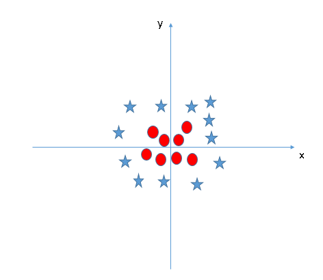
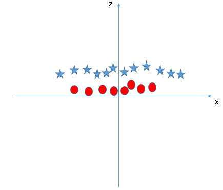
After the data points are “shockedâ€, the stars and circles appear on the Z-axis with a clear decision boundary. It is represented in the figure above as a two-dimensional line. Here are a few points to note:
All values ​​of Z are positive because it is the sum of squares of X and Y;
In the original image, the distribution of circles is closer to the origin of the axes than the stars, which is why their values ​​on the Z-axis are lower.
In SVM, we can easily obtain such a linear hyperplane between two types of data by increasing the space dimension, but another problem that needs to be solved is whether new features such as Z = X2 + Y2 have to be owned by us. Manual design? No, there is a function in the SVM called kernel that maps low-dimensional input into high-dimensional space and linearly separable the original linearly indivisible data. We also call them kernel functions.
Kernel functions are mainly used for nonlinear separation problems. In short, it automatically performs some very complex data transformations and then finds the process of separating the data based on the tags or outputs you define.
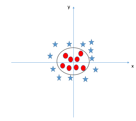
When we compress the data points back from 3D to 2D, the hyperplane becomes a circle:
3. How to implement SVM in Python and R
In Python, scikit-learn is a very convenient and powerful machine learning algorithm library, so we can find SVM directly in scikit-learn.
#Import Library
From sklearn import svm
#Assumed you have, X (predictor) and Y (target) for training data set and x_test(predictor) of test_dataset
# Create SVM classification object
Model = svm.svc(kernel='linear', c=1, gamma=1)
# there is various option associated with it, like changing kernel, gamma and C value. Will discuss more # about it in next section.Train the model using the training sets and check score
Model.fit(X, y)
Model.score(X, y)
#Predict Output
Predicted= model.predict(x_test)
For the R language, the e1071 package can be used to easily create an SVM with helper functions and code for the Naive Bayes classifier, much the same as Python.
#Import Library
Require(e1071) #Contains the SVM
Train <- read.csv(file.choose())
Test <- read.csv(file.choose())
# there are various options associated with SVM training; like changing kernel, gamma and C value.
# create model
Model <- svm(Target~Predictor1+Predictor2+Predictor3,data=Train,kernel='linear',gamma=0.2,cost=100)
#Predict Output
Preds <- predict(model,Test)
Table(preds)
How to adjust SVM parameters
In machine learning, tuning is an effective way to improve model performance. Let's take a look at the available parameters in the SVM.
sklearn.svm.SVC(C=1.0, kernel='rbf', degree=3, gamma=0.0, coef0=0.0, shrinking=True, probability=False, tol=0.001, cache_size=200, class_weight=None, verbose= False, max_iter=-1, random_state=None)
Here we introduce only a few important parameter adjustment methods.
Kernel: We have already introduced what the kernel is. We can pick various functions about it: linear, RBF kernel, poly function, etc. (default is RBF kernel). For the nonlinear hyperplane, the last two kernel functions have significant effects. Here are a few examples:
Example 1: Linear Kernel Function
Import numpy as np
Import matplotlib.pyplot as plt
From sklearn import svm, datasets
# import some data to play with
Iris = datasets.load_iris()
X = iris.data[:, :2] # we only take the first two features. We could have
# avoid this ugly slicing by using a two-dim dataset
y = iris.target
# we create an instance of SVM and fit out data. We do not scale our
# data since we want to plot the support vectors
C = 1.0# SVM regularization parameter
Svc = svm.SVC(kernel='linear', C=1,gamma=0).fit(X, y)
# create a mesh to plot in
X_min, x_max = X[:, 0].min() - 1, X[:, 0].max() + 1
Y_min, y_max = X[:, 1].min() - 1, X[:, 1].max() + 1
h = (x_max / x_min)/100
Xx, yy = np.meshgrid(np.arange(x_min, x_max, h),
Np.arange(y_min, y_max, h))
Plt.subplot(1, 1, 1)
Z = svc.predict(np.c_[xx.ravel(), yy.ravel()])
Z = Z.reshape(xx.shape)
Plt.contourf(xx, yy, Z, cmap=plt.cm.Paired, alpha=0.8)
Plt.scatter(X[:, 0], X[:, 1], c=y, cmap=plt.cm.Paired)
Plt.xlabel('Sepal length')
Plt.ylabel('Sepal width')
Plt.xlim(xx.min(), xx.max())
Plt.title('SVC with linear kernel')
Plt.show()
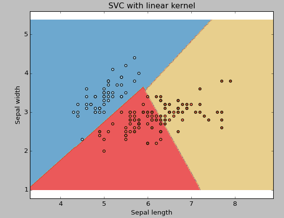
Example 2: RBF kernel function
Change the kernel function type to rbf and observe the change from the graph.
Svc = svm.SVC(kernel = 'rbf', C = 1, gamma = 0).fit(X,y)
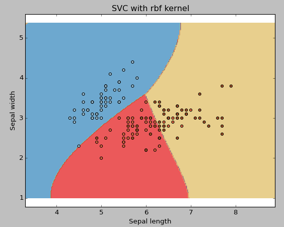
If you have a large number of features (> 1000), I suggest that you choose linear kernels because they are more likely to be linearly separable in higher dimensional space. In addition, that rbf is a good choice, but don't forget to cross-validate its parameters to avoid overfitting.
Gamma: The nuclear coefficient of rbf, poly, and sigmoid. The higher the gamma value, the more difficult the model is to fit the training dataset, so it is also a factor that causes overfitting.
Example 3: gamma = 0.01 and 100
Svc = svm.SVC(kernel = 'rbf', C = 1, gamma = 0).fit(X,y)

C: The penalty parameter C of the error term, which also controls the trade-off between the smoothness of the decision boundary and the correct classification training point.
Example 4: C = 100 and 1000

From beginning to end, we must remember to use cross-validation to effectively combine these parameters to prevent overfitting of the model.
5. Advantages and disadvantages of SVM
advantage
Good results, clear classification boundaries;
Particularly effective in high-dimensional space;
It is very effective when the spatial dimension is larger than the number of samples;
It uses a subset of training points (support vectors) in the decision function, so it has a small memory footprint and high efficiency.
Shortcomings
If the amount of data is too large or the training time is too long, SVM will perform poorly;
If there is a lot of noise in the data set, SVM does not work well;
The SVM does not directly calculate the probabilistic estimates, so we have to perform multiple cross-validations at too high an expense.
summary
This article describes what a support vector machine, the working principle of SVM, how to implement SVM in Python and R, how to adjust parameters and its advantages and disadvantages. I hope readers will try it out after reading. Don't be influenced by the saying “Do you still need to learn svm?†in recent years. The classic algorithm always has its own valuable points. It is also when you enter the company interview. A hot topic.
If you don't know where to begin, you can try to do this topic:
Which is the most welcome kid laptop for entertainment and online learning? 10.1 inch laptop is the best choice. You can see netbook 10.1 inch with android os, 10.1 inch windows laptop, mini laptop 10.1 inch 2 in 1 windows, 10.1 inch 2 In 1 Laptop with android os. Of course, there are various matches of memory and storage, 2 32GB or 4 64GB. Our suggestion is that 10.1 inch android 32GB laptop, 10.1inch 32GB or 64GB Solid State Drive windows laptop. Except 10.1 inch Student Laptop , there are 11 Inch Laptop, 15.6 Inch Laptop, 14 Inch Laptop , also option here.
Besides, other advantages you can see on 10.1inch Budget Laptop For Students, for example, lightweight, competitive cost, portability, Android or Windows OS, rich slots, energy saving cpu, etc.
As a professional manufacturer, can provide free custom service, like mark client`s logo on laptop cover, opening system, inner color box, manual, boot. Produce as your special requirement on parameters, preinstall apps needed, etc. What you need to do is very simple, confirming PI, including price, delivery time, parameters, etc.
10.1 Inch Laptop,Netbook 10.1 Inch,10.1 Inch 2 In 1 Laptop,10.1 Inch Windows Laptop,Mini Laptop 10.1 Inch
Henan Shuyi Electronics Co., Ltd. , https://www.shuyitablet.com