Constructing a hidden layer neural network using SQL query statements

The SQL we are familiar with is a database query that makes it easy for developers to perform efficient operations on large data. However, this article builds a simple three-layer fully-connected network by nesting SQL query statements from another angle. Although the nesting of statements is too deep and cannot be efficiently calculated, it is still a very interesting experiment.

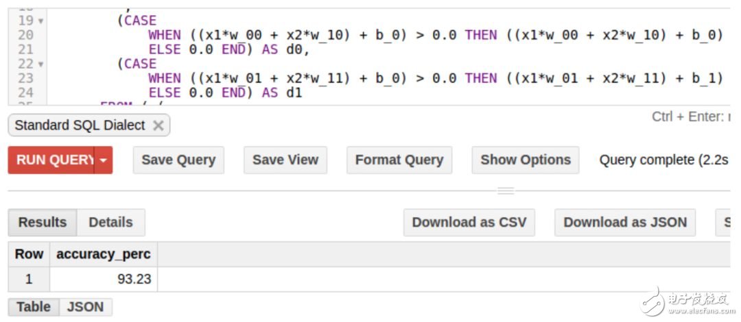
In this article, we will implement a neural network with a hidden layer (and with ReLU and softmax activation functions) purely in SQL. These neural network training steps include forward propagation and back propagation, which will be implemented in a single SQL query statement in BigQuery. When it's running in BigQuery, we're actually doing distributed neural network training on hundreds of servers. It sounds great, right?

That said, this interesting project is used to test the limitations of SQL and BigQuery while looking at neural network training from the perspective of declarative data. This project does not consider any practical application, but in the end I will discuss some practical research implications.

Let's start with a simple classifier based on neural networks. It has an input size of 2 and an output of two. We will have a single hidden layer with a dimension of 2 and a ReLU activation function. The second classification of the output layer will use the softmax function. The steps we will follow when implementing the network will be the SQL-based version of Python shown in the Karpathy's CS231n guide (https://cs231n.github.io/neural-networks-case-study/).

model

The model has the following parameters:

Input to the hidden layer

Weight matrix of W: 2&TImes; 2 (element: w_00, w_01, w_10, w_11)

B: offset vector of 2&TImes;1 (element: b_0, b_1)

Hidden to the output layer

Weight matrix of W2: 2&TImes;2 (element: w2_00, w2_01, w2_10, w2_11)

B2: offset vector of 2&TImes;1 (element: b2_0, b2_1)

The training data is stored in a BigQuery table. The inputs and outputs for columns x1 and x2 are as follows (table name: example_project.example_dataset.example_table)

As mentioned earlier, we implement the entire training as a single SQL query statement. After the training is completed, the value of the parameter will be returned through the SQL query statement. As you might guess, this will be a layered nested query, and we will build it step by step to prepare this query. We will start with the innermost subquery and then add the nested outer layers one by one.

Forward propagation

First, we set the weight parameters W and W2 to random values ​​that follow a normal distribution, and set the weight parameters B and B2 to zero. Random values ​​for W and W2 can be generated by the SQL itself. For the sake of simplicity, we will generate these values ​​externally and use them in SQL queries. The internal subquery used to initialize the parameters is as follows:

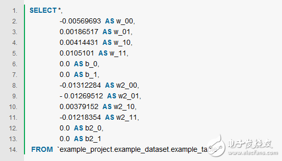
Note that the table example_project.example_dataset.example_table already contains columns x1, x2, and y. The model parameters will be added as additional columns to the results of the above query.

Next, we will calculate the activation value of the hidden layer. We will use the vector D containing the elements d0 and d1 to represent the hidden layer. We need to perform the matrix operation D = np.maximum(0, np.dot(X, W) + B), where X is the input vector (elements x1 and x2). This matrix operation involves multiplying the weight W by the input X, plus the offset vector B. The result is then passed to the nonlinear ReLU activation function, which will set the negative value to zero. The equivalent query in SQL is:

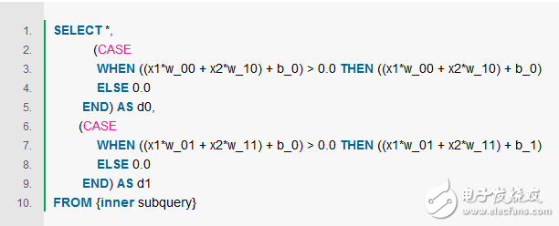
The above query adds two new columns d0 and d1 to the results of the previous internal subquery. The output of the above query is as follows.

This completes a conversion from the input layer to the hidden layer. Now we can perform the conversion from the hidden layer to the output layer.

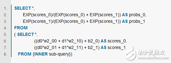
First, we will calculate the value of the output layer. The formula is: scores = np.dot(D, W2) + B2. Then, we will use the softmax function on the calculated values ​​to get the predicted probability of each class. The equivalent subquery inside SQL is as follows:

First, we will use the cross entropy loss function to calculate the total loss of the current prediction. First, calculate the negative value of the logarithm of the correct class prediction probability in each sample. The cross entropy loss is simply the average of the values ​​in these X and Y instances. The natural logarithm is an increasing function, so it is intuitive to define the loss function as a negative correct class predictive probability log. If the prediction probability of the correct class is high, the loss function will be low. Conversely, if the prediction probability of the correct class is low, the loss function value will be high.

In order to reduce the risk of overfitting, we will also increase L2 regularization. In the overall loss function, we will contain 0.5*reg*np.sum(W*W) + 0.5*reg*np.sum(W2*W2), where reg is a hyperparameter. Including this function in the loss function will punish the larger of those weight vectors.

In the query, we also calculate the number of training samples (num_examples). This is useful for subsequent calculations of the average. The statement for calculating the overall loss function in an SQL query is as follows:

Back propagation

Next, for backpropagation, we will calculate the partial derivative of each parameter for the loss function. We use the chain rule to calculate layer by layer from the last layer. First, we will calculate the gradient of the score by using the derivative of the cross entropy and the softmax function. The opposite query is:

In the above, we calculated the score with scores = np.dot(D, W2) + B2. Therefore, based on the partial derivative of the fraction, we can calculate the gradient of the hidden layer D and the parameters W2, B2. The corresponding query statement is:

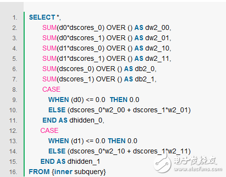
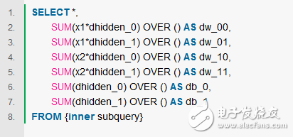
Similarly, we know that D = np.maximum(0, np.dot(X, W) + B). Therefore, through the partial derivative of D, we can calculate the derivatives of W and B. We do not need to calculate the partial derivative of X because it is not a parameter of the model and does not have to be calculated by other model parameters. The query for calculating the partial derivatives of W and B is as follows:

Finally, we update the operations using the derivatives of W, B, W2, and B2. The calculation formula is param = learning_rate * d_param , where learning_rate is a parameter. To reflect L2 regularization, we add a regular term reg*weight when calculating dW and dW2. We also remove cached columns such as dw_00, correct_logprobs, etc., which were created during subqueries to hold training data (x1, x2, and y columns) and model parameters (weights and offsets). The corresponding query statement is as follows:

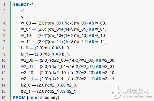
This involves an entire iterative process of forward and reverse propagation. The above query will return the updated weights and offsets. Some of the results are as follows:

In order to perform multiple training iterations, we will repeat the above process. It's enough to do this with a simple Python function, the code link is as follows: https://github.com/harisankarh/nn-sql-bq/blob/master/training.py.

Because of the multiple nesting and complexity of query statements, multiple system resources are anxious when executing queries in BigQuery. BigQuery's standard SQL extensions are more scalable than traditional SQL languages. Even for standard SQL queries, it is difficult to perform more than 10 iterations for a dataset with 100k instances. Because of resource constraints, we will use a simple decision boundary to evaluate the model, so that we can get better accuracy after a small number of iterations.

We will use a simple data set with input X1, X2 obeying the standard normal distribution. The binary output y simply determines if x1 + x2 is greater than zero. In order to train 10 iterations faster, we use a larger learning rate of 2.0 (Note: such a large learning rate is not recommended for practical use and may result in divergence). The model parameters obtained by executing the above 10 iterations of the above statement are as follows:

We will use Bigquery's function save to table to save the result to a new table. We can now perform a reasoning on the training set to compare the difference between the predicted and expected values. The query fragment is in the following link:

Https://github.com/harisankarh/nn-sql-bq/blob/master/query_for_prediction.sql.

With only 10 iterations, our accuracy rate is 93% (the test set is similar).

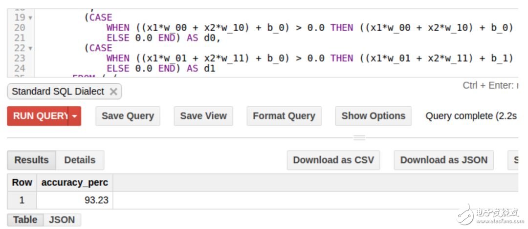
If we add the number of iterations to 100 times, the accuracy rate is as high as 99%.

optimization

The following is a summary of the project. What inspired us? As you can see, resource bottlenecks determine the size of the data set and the number of iterations. In addition to praying for Google's open resource cap, we have the following optimizations to solve this problem.

Creating intermediate tables and multiple SQL statements can help increase the number of iterations. For example, the results of the first 10 iterations can be stored in an intermediate table. The same query statement can be based on this intermediate table when it performs the next 10 iterations. So, we performed 20 iterations. This method can be used repeatedly to handle larger query iterations.

Instead of adding external queries at each step, we should use nesting of functions whenever possible. For example, in a subquery, we can compute both scores and probs instead of using 2 levels of nested queries.

In the above example, all intermediate items are retained until the last outer query is executed. Some of these items, such as correct_logprobs, can be removed earlier (although the SQL engine may perform such optimizations automatically).

Try to apply user-defined functions. If you're interested, you can take a look at the project model for this BigQuery user-defined function (but you can't use SQL or UDFs for training).

significance

Now let's take a look at the deeper meaning of a distributed SQL engine based on deep learning. One limitation of the SQL warehouse engine such as BigQuery and Presto is that the query operation is performed on the CPU instead of the GPU. It is interesting to study GPU-accelerated database query results such as blazingdb and mapd. A simple research approach is to use a distributed SQL engine to perform queries and data distribution, and to use the GPU to accelerate the database to perform local calculations.

Taking a step back, we already know that it is difficult to perform distributed deep learning. The distributed SQL engine has had a lot of research work in decades, and it has produced technologies such as query planning, data partitioning, operation placement, checkpoint setting, and multi-query scheduling. Some of them can be combined with distributed deep learning. If you are interested in this, please take a look at this paper (https://sigmodrecord.org/publications/sigmodRecord/1606/pdfs/04_vision_Wang.pdf), which covers a wide range of distributed databases and distributed deep learning. Research discussion.

Busbar Heat Shrink Tubing

Bushing Cover For Busbar provide electric insulation protection heat shrink cover for busbar.

Supply Protection and Insulation for Switchboard and Substation.

Provide Insulation and Enhancement for Busbar.

Features:

1.Suitable for 1-35KV.

2.Radiation cross linking materials (Polyolefin or EPDM rubber ).

3.Quick and easy installation.

4.Avoid short circuit and leakage.

5.Facilitate routine inspection and maintenance.

6.Resistant to moisture and dust.

7.Meet RoHS Stand.

8.Customized

We are the professional manufacturer of Electrical Tapes,Insulating Tape and Heat Shrink Tubing in China for more than 25 years,if you want to know more information about our company and products, please visit our website.

Busbar Heat Shrink Tubing,Busbar Heat Shrink Sleeve,Busbar Heat Shrink,Heat Shrink Busbar Insulation

CAS Applied Chemistry Materials Co.,Ltd. , https://www.casac1997.com